Background

When I was looking for a node to write about, I searched for something that was the right combination of not being trivial but also being something that I could pop out in a relatively quick blog post. It ended up being my third post (the visualizations were a pain).

I landed on my DXT1 compression node. DXT1 is a lossy compression algorithm that is still, to my knowledge, sometimes used when compressing textures for games. I work mostly in Unity, where that sort of thing is a texture setting that you rarely fiddle with. It’s also kind of a weird pick for an image pipeline where I’m mostly trying to make an image look different in a stylistic way, but we’ll get to where I landed with it, which is moderately interesting.

For now, this is what my DXT1 node does with the most authentic settings. If you click (or press) and hold on the image, it’ll show the original for comparison.

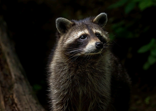
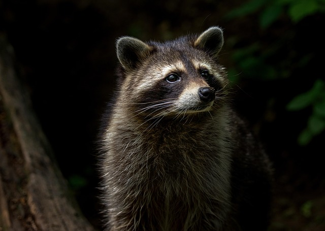
With this image, it does a fairly good job of not losing much detail. It’s most noticeable in the chest fur, where it turns from brown into more of a gray, losing some of the dark colors in the background, and losing some details around the whiskers.

Why Use DXT1

Well, it’s a compression algorithm. I’m not sure how it stacks up to jpeg or png, but against raw RGB888, it fares well. RGB888 is 24 bits (3 bytes) per pixel (8 + 8 + 8). A 4x4 RGB888 chunk would be 384 bits (48 bytes). A DXT1 chunk, on the other hand, is just 64 bits (8 bytes). That’s a sixth of the size, and only 4 bits per pixel.

Additionally, since DXT1 is a fixed byte size per chunk, you can access an arbitrary chunk in constant time. This is something that neither jpg nor png generally support.

Now, this is sort of comparing an apple to an orange. Neither jpg or png are used in high performance game engines.

My understanding is that DXT1 is still used often, as long as none of the following apply:

• The texture is loss-sensitive and viewed from up close (you probably wouldn’t use this on a scaled up UI texture).
• Artifacting within 4x4 chunks would be noticeable (you’ll see some cases here, this is basically my reason for making this node).
• RGB565 is too coarse for the data (you’ll see why that could occur later).

The worst fit is likely normal maps. RGB565 is coarse for data that isn’t really color (channels represent X/Y/Z), and all four colors in a chunk have to lie on a line in RGB space (which is often very not true for normal maps).

How DXT1 Works

DXT1¹ is a specification² for an image compression format.

The high level of how it works is simple: the image is split up into 4x4 chunks, each of which can contain four distinct colors. These colors are two boundary colors and, depending on whether the chunk contains transparency or not, either two interpolated colors or one interpolated color and one fully transparent pixel.

Color Interpolation

Now, the point of compressing an image is to make it smaller. To do that, DXT1 gives up flexibility in the nature of the colors that can be expressed.

The boundary colors³ are the only two colors that you can directly specify per chunk. The color of each pixel is specified by the number 0-3, which indicates boundary color 1 $c_{b1}$, boundary color 2 $c_{b2}$, or two interpolated colors.

For chunks without transparency, these interpolated colors are $(2c_{b1} + c_{b2}) / 3$ and $(c_{b1} + 2c_{b2}) / 3$. For chunks with transparency, it’s $(c_{b1} + c_{b2}) / 2$ and a fully transparent pixel.⁴

A Diversion into Color Bits

Generally when I think of colors on the computer, I’m thinking of the good ol’ 8 bits (256 values) per channel colors. The kind you’d represent with a hex code, like #00BFFF . This is called RGB888, indicating that each of the red, green, and blue, channels contains eight bits of data.

The colors directly specified on disk for the DXT1 compression format are not stored in RGB888 or RGBA8888. As opposed to RGB888, which can represent around 16.7 million colors, DXT1 uses a RGB565 format, which can represent 65,536 colors. RGB565 means that the red and blue channel are represented using 5 bits (32 distinct values) and the green channel is represented using 6 bits (64 distinct values).

This causes obvious banding on all of the color gradients, as visualized below.

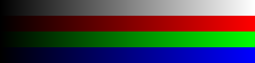
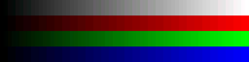
Something a bit more subtle is that this introduces either a green or magenta tint in portions of the grayscale ramp. Gray should theoretically mean all colros are equal, but since green is quantized on a finer grid, it will sometimes get rounded higher (a green tint) or lower (a magenta tint).

Why did they pick an extra bit in the green channel? Well, first of all, it has to go somewhere; data is generally stored in multiples of 8 and sixteen doesn’t split evenly into three parts. 5 + 6 + 5 = 16 is as close as you can get. This is given to green as, allegedly, humans are better at determining differences in green than red or blue. I’m sure there’s a bunch of science backing this up—I didn’t bother to look into it. If I look at the RGB888 ramp, I can spot the differences in values a little bit easier than I can with red or especially blue, so I believe it.

Packing the Data

Earlier I said that colors adding up to 16 bits had some nice properties for packing DXT1. If you have sixteen (4x4) pixels to represent, four colors to choose from, and two 16-bit boundary colors, that means it’ll fit nicely in 64 bits:

$$\underbrace{16 \times 2}_{\text{pixel indices}} + \underbrace{2 \times 16}_{\text{boundary colors}} = 64\ \text{bits}$$

Having it be a fixed size but also byte-aligned makes seeking easy, which is nice if you’re trying to look up data partway through a texture.

Eagle-memoried readers will notice that this doesn’t allow specifying which mode the chunk is in: opaque or transparent. However, we actually have an additional bit’s worth of data we can squeeze into the format: the ordering of the boundary colors. If the first boundary color is greater than the second (remember that these are represented using numbers), it’s in opaque mode (the 33% and 66% colors). If the first boundary color is less than or equal to the second, it’s in transparent mode (the 50% and transparent colors).

Interpolating the Bits

The boundary colors are stored in RGB565, but that’s only half of the palette. Because the two other colors are computed from them, they’re never written to any dis in any explic color format—which means they aren’t constrained to RGB565. This means that DXT1 textures can actually show colors with far more granularity than can be represented with 16 bits!⁵

Picking the Boundary Colors

DXT1 is just a format for representing images. It doesn’t actually tell you how to pick the colors. That means that we need to figure it out ourselves. Note that transparent pixels are not considered in any of my algorithms below. Not a requirement, just how I did it.

Luminance

In my first stab at it, I decided to pick the pixels with the highest and lowest luminance and treat them as the boundary colors. I compute luminance with the following equation:

$$L = 0.299R + 0.587G + 0.114B$$

Here’s a rough visualization of the algorithm (in RG space instead of RGB to make it easier to visualize).

For a first stab in the dark, this actually works fairly well.⁶

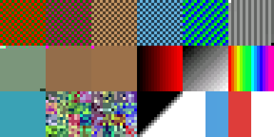
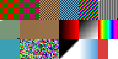
This performs poorly when your luminance outliers are different colors than the rest of the data set.

RGB Bounding Box

In my next attempt, I decided to actually look at what people did in the wild. Several encoders used a RGB bounding box approach as their performant, low quality approach. What it does is find the maximum and minimum red, green, and blue values (examining channels independently) and use those min values and max values as the endpoints. It’s probably faster than my luminance check (no floating point multiplication), but also has more easily reproducible undesirable cases.

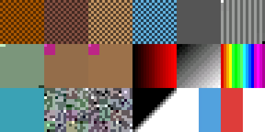
RGB bounding box has some trivially obvious failure modes that can be seen here—you can force out the boundaries to be the entire color space, resulting in gray chunks. Color from a single pixel can also bleed out into the chunk.

Principal Component Analysis (PCA)

As far as I could tell, PCA formed the basis of most high-quality DXT1 encodings.⁷

I’ve always struggled once people bust out the math notation,⁸ so understanding this was somewhat tricky to wrap my head around.⁹ Here’s the pitch of PCA: plot all sixteen pixels of a chunk as points in 3D space, one axis per color channel. PCA finds the single line through that cloud of points that the colors are most stretched along. The two pixels farthest apart along that line are used as our boundaries.

The reason this works for DXT1 is that the interpolated colors lie on a line between the two boundary colors. If the chunk’s actual colors happen to lie close to some line in RGB space, then picking endpoints along that exact line means our four representable colors will be close to every real pixel. The RGB bounding box approach also defines a line (the diagonal of the bounding cube), but it’s only the right line if the colors happen to vary along that diagonal.¹⁰

The visualization below walks through the steps. It may be worth referring back to as we work through the math.

Solving PCA

First, a legend of all the terms. Probably best to skip over this and consult it as they come up:

• $\mathbf{p}$: a single pixel in the chunk (a vector), with components $(p_\mathrm{r}, p_\mathrm{g}, p_\mathrm{b})$.
• $n$: the number of pixels in the chunk (16 for a standard 4x4 DXT1 chunk).
• $\sum_p$: a sum that runs over every pixel $\mathbf{p}$ in the chunk.
• $\lVert \mathbf{u} \rVert$: the magnitude (length) of a vector $\mathbf{u}$.
• $\mathbf{m}$: the mean color (a vector), with components $(m_\mathrm{r}, m_\mathrm{g}, m_\mathrm{b})$. The average of all the pixels.
• $\mathbf{p}_\mathrm{f}$: the farthest pixel from the mean.
• $\mathbf{C}$: the 3×3 covariance¹¹ matrix built from the chunk’s pixels. An entry $C_{xy}$ describes how channels $x$ and $y$ vary together. e.g. $C_{\mathrm{rg}}$ is the red/green entry and $C_{\mathrm{rr}}$ red/red.
• $\mathbf{v}$: This is the best fit line. Mathematically, it’s the principal eigenvector of $\mathbf{C}$.
• $s_p$: The projection of pixel $\mathbf{p}$ onto the best fit line. A single number describing how far along the line that pixel sits.

Figuring out what we need

We can plot the chunk’s sixteen pixels plotted as points in 3D space, one axis per color channel. PCA computes a best fit line through that point cloud that the pixels compose. The pixels at the two extreme ends of that line are our boundary colors.

Conceptually, I think it’s simpler to work backwards from what we want (the boundary colors) to how we get what we want. As mentioned above, we plan on getting these boundary colors from the best fit line. We can do this by computing the dot product of the pixel’s offset from the mean ($\mathbf{m}$) against a vector that defines the best fit line. The pixels with the lowest and highest values are our boundary colors.

Okay, so now we know that we need the mean color $\mathbf{m}$ and the best fit line. Determining $\mathbf{m}$ is easy: compute the average color of the chunk by averaging each channel across all pixels.

Determining the best fit line is more complicated. We need the principal eigenvector $\mathbf{v}$ of the covariance matrix $\mathbf{C}$. Given $\mathbf{C}$, determining $\mathbf{v}$ is not complicated. We can use power iteration to turn a starting vector¹² into $\mathbf{v}$.¹³ Picking the vector determined by subtracting the farthest point from the mean gives a good start.

Now we just need $\mathbf{C}$, the 3x3 matrix describing how channels vary together. For each channel pair (e.g. $C_{\mathrm{rg}}$), subtract the mean from each of the two channels, multiply the two results, and sum across every pixel in the chunk. And that’s it! We’ve worked ourselves back to the starting position.

If that didn’t make sense, maybe the following forward approach (with equations) will be easier to follow.

Laying out the equations

Now let’s solve this forward to get to the boundary colors.

Mean color, computed component-wise across all pixels:

$$\mathbf{m} = \frac{1}{n} \sum_p \mathbf{p}$$

3x3 Covariance matrix $\mathbf{C}$ formula. One computation for each channel pair, with $x$ and $y$ each ranging over $\{\mathrm{r}, \mathrm{g}, \mathrm{b}\}$:

$$C_{xy} = \sum_p (p_x - m_x)(p_y - m_y)$$

$\mathbf{C}$ is symmetric along the diagonal ($C_{xy} = C_{yx}$), so only six of the nine entries are unique:

$$\mathbf{C} = \begin{bmatrix} C_{\mathrm{rr}} & C_{\mathrm{rg}} & C_{\mathrm{rb}} \\ C_{\mathrm{rg}} & C_{\mathrm{gg}} & C_{\mathrm{gb}} \\ C_{\mathrm{rb}} & C_{\mathrm{gb}} & C_{\mathrm{bb}} \end{bmatrix}$$

We use power iteration to extract the best fit line. Normalization (dividing by its magnitude) occurs to prevent $\mathbf{v}$ from getting big enough to introduce floating point error. Seed $\mathbf{v}_0$ with the unit vector from $\mathbf{m}$ toward the pixel farthest from $\mathbf{m}$—call that pixel $\mathbf{p}_\mathrm{f}$:

$$\mathbf{v}_0 = \frac{\mathbf{p}_\mathrm{f} - \mathbf{m}}{\lVert \mathbf{p}_\mathrm{f} - \mathbf{m} \rVert}$$

A constant seed like $(1, 1, 1)$ also worked well, but if it lands nearly perpendicular to the principal eigenvector, I think it could cause problems.¹⁴ Seeding with the farthest pixel will often start us off from a good place. Then iterate:

$$\mathbf{v}_{k+1} = \frac{\mathbf{C}\mathbf{v}_k}{\lVert \mathbf{C}\mathbf{v}_k \rVert}$$

After 12 iterations (chosen empirically), it appeared to converge well enough in the cases I tried.

Project each pixel onto $\mathbf{v}$ to get a scalar position along the line:

$$s_p = (\mathbf{p} - \mathbf{m}) \cdot \mathbf{v}$$

The two boundary colors are the pixels at the smallest and largest values of $s_p$.

The Results

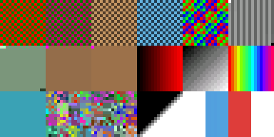
The failure mode is most obvious here in the top right (as it was for RGB bounding box), which is ironic—that’s the case I made to try to shut the failing of luminance. A single extra blue pixel pulls the best fit line toward blue, which brings the rest of the chunk with it. In cases where it does have it, it leans toward red or green. Across the whole square, PCA represents it better, but it looks less cohesive than luminance does.

Thinking Through Optimizations

As I mentioned at the start, DXT1 doesn’t specify how you generate the boundary colors or choose whether to encode it in opaque or transparent mode.

A naive approach would be to take the darkest pixel and take the brightest pixel (maybe computing the luminance of each) and choose those as your boundary colors. If there’s transparency, put it in transparent mode. Otherwise, put it in opaque mode. There is, however, some room for improvement.

Picking Better Boundaries

Let’s assume we have a chunk that represents a piece of gray fabric.

It has:

• Seven pixels of light thread: gray 156 (#9C9C9C )
• Seven pixels of dark thread: gray 100 (#646464 )
• One pixel slightly darker (a shadow): gray 75 (#4B4B4B )
• One pixel slightly lighter (a highlight): gray 181 (#B5B5B5 )

If we naively pick the endpoints, gray 75 (#4B4B4B ) and gray 181 (#B5B5B5 ), we’d get the interpolated colors gray 110 (#6E6E6E ) and gray 146 (#929292 ).

This would leave 2 pixels with 0 error and 14 pixels with 10 error.

However, what if we expanded the boundary pixels so that the interpolated pixels hit our target?

With the endpoints of gray 44 (#2C2C2C ) and gray 212 (#D4D4D4 ), our interpolated colors exactly match our targets, gray 156 (#9C9C9C ) and gray 100 (#646464 ).

This leaves 2 pixels with 25 error, 14 pixels with 0 error, and a resulting image much closer to what we want. The outliers are more outliery, which isn’t great, but most of the texture is closer.

By my understanding, some of the algorithms used to compress textures do just this, although my implementation does not. There’s some artistry to this; I could imagine artists wanting to go in to tweak some of these numbers on more important textures.¹⁵

Choosing a Different Mode

Usually more colors is better, right? Not necessarily.

You probably already have something in mind, but here’s a concrete example. A leaf, with the chunk primarily being #789678 , #C8F0C8 , and #283C28 .¹⁶

With the opaque ordering, you get the interpolated colors #5D785D and #93B493 . Both of those would probably look good enough, but can we do better?

If you interpolate halfway between the two boundary colors (#C8F0C8 and #283C28 ), you get #789678 which just so happens to be a perfect match for our third color.¹⁷ So despite not having any transparency, we can structure the color order to pretend that we do to get some closer matches.

This one my matching algorithm does do, as it’s not much more work to do so (programmatically).

Comparing Approaches

So, we’ve established that I have three different heuristics for choosing the boundary colors (luminance, RGB bounding box, PCA) and two color mode choices (opaque vs. transparent). As we saw in the comparison, none of them win every time. So, why not make them fight?

First, we need to decide a heuristic for what makes a color encoding best. I use a sum of squared errors approach, which is quite simple. For each pixel, I find the closest color, compute the difference of each channel, square each distance, and sum the error across all the pixels. The approach with the lowest error wins. Errors are squared because ten pixels differing by one unit is better than one pixel differing by ten units.

In short:

1. Run each permitted strategy to get an endpoint pair.
2. For each candidate, convert the endpoints to RGB565 and compute the interpolated palette colors for both 4-color and 3-color modes.¹⁸
3. For every variant, sum the squared error across all opaque pixels in the chunk.
4. Use the (endpoints, mode) combination that has the lowest total error.

This is slower than any of the approaches on their own, but this is not one of the nodes that is meaningfully slow, so I haven’t found it worth trying to optimize it.

In the Pipeline

Everything above describes a working DXT1 encoder. However… I’m not actually using it as one. I take all that compressed output and immediately bake it into a normal RGBA8888 image.

In that way, this deviates greatly from what any DXT1 approach does in practice, and makes it more or less useless for using as a DXT1-compressed image generator. While you probably could figure out which boundary colors a chunk is derived from, I imagine it’d be slower than just re-encoding the source image.

You might be looking up at the image at top and saying, “yeah, it’s slightly different, but why bother?” That’s a reasonable comment.

However, there’s no real reason from an algorithmic standpoint that chunks need to be 4x4. They could be 64x64 or 128x2 or even cover the whole image.

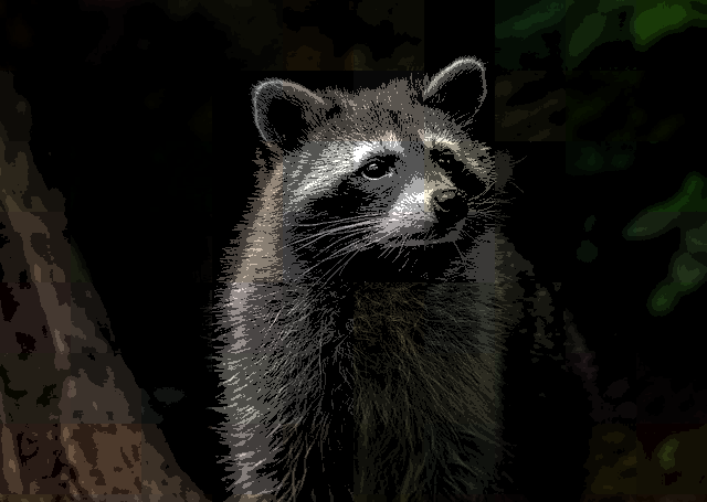
Is this worth it as a node? I like the appearance with the large chunk size, and it offers an interesting take on a four level posterization, but the lack of control over the number of colors makes it rather limited.

For the artistic use I landed on, my first luminance approach would have been sufficient, but learning about two more mathematical approaches was an interesting, if sometimes frustrating, way to dip my toe back into more mathematical waters.

Picking DXT1 as the first node¹⁹ I write up here was borne out of practicality. It was in the sweet spot between trivial and utterly complex, which made it a balanced node to write about. The node has its own weird place in the pipeline, but adding nodes like this was part of the reason I undertook the project in the first place—I want to do weird transformations that traditional art software wouldn’t.