
Making a Bad Image Pipeline: Kuwahara Filter
Background
On March 31st, I wanted to make a pixel art version of my Discord avatar as a fun little change for April Fools day. Since I’m lazy and not good at pixel art, this quickly turned into wanting something that looked like pixel art (e.g. scaled down, restricted palette). I tried using color indexing in Photoshop, but it didn’t give me the feel that I wanted. I then searched online for some available web tool. Ironically, I can’t actually remember what service I did use for this, but I ended up unsatisfied by the results.
I was also curious about the underlying mechanisms used in generating the results—I have some basic knowledge of pixel art, so I know how color matching to get pixels to match a palette and dithering generally work, but I wanted to understand the effect that color matching algorithms and dithering algorithms could have on the results.
Dithering and palettization get a lot of attention online, and they’re also a lot of work to explain well, so I’m going to start with a simpler node supported by my pipeline: the Kuwahara filter.
The Kuwahara Filter is, unsurprisingly, named after someone named Kuwahara: Michiyoshi Kuwahara, who worked on medical imaging in the 70s and 80s. This filter was allegedly a way of reducing noise on medical imagery. I’d like to know more, but unfortunately, all the discussion of that (a few blog posts, wikipedia) appears to be unsourced, so I’d be reluctant to spread it over more of the internet if it’s not true.
Regardless, the Kuwahara filter is a noise-reduction filter that preserves edges. Its effect can be seen on the raccoon image below. If you click (or press) and hold on the image, it’ll show the original for comparison.
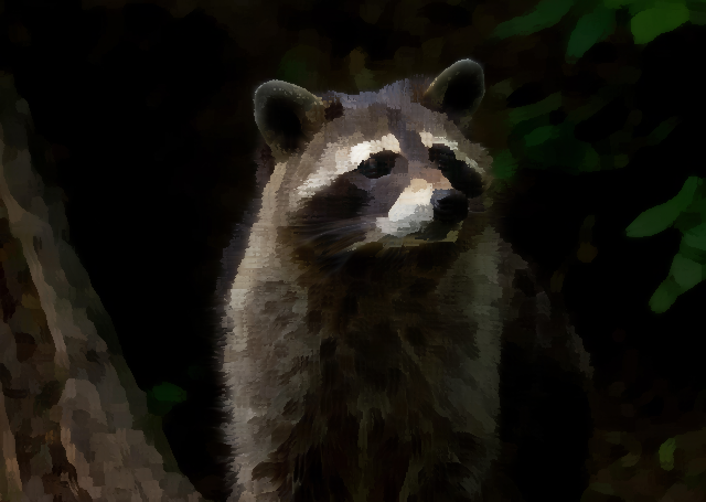
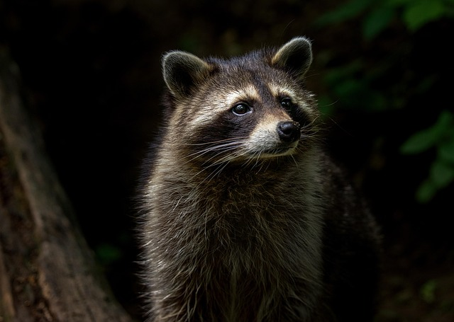
As you can see above, the filter gives a vague facsimile of being painted with actual brushstrokes. It lacks the texture or intentionality of brush strokes, but it’s something easy to reach for if you want to make your VN backgrounds look slightly less like images you snagged off the web.
How it Works
First, we calculate the luma of each pixel in the image. Luma is a measure of the brightness of an image, and it’s just a matter of scaling the RGB channels by different weights. I use the Rec. 601 luma computation:1
$$L = (0.299R + 0.587G + 0.114B)$$
This gives us luminance in a range of 0-255. Pixels here will use the format $L_{xy}$. The RGB pixels of the image themselves will be referred to with $I_{xy}$.
Kuwahara iterates over every pixel $I_{xy}$ in the image. It processes four squares around it: for a window of radius $r$ centered on the pixel, the window is divided into four overlapping quadrants that share the center row and column. The center pixel $I_{xy}$ itself belongs to all four. The grid below shows quadrant membership for a radius 2 (5x5) window:
| -2 | -1 | 0 | 1 | 2 | |
|---|---|---|---|---|---|
| -2 | 1 | 1 | 12 | 2 | 2 |
| -1 | 1 | 1 | 12 | 2 | 2 |
| 0 | 13 | 13 | 1234 | 24 | 24 |
| 1 | 3 | 3 | 34 | 4 | 4 |
| 2 | 3 | 3 | 34 | 4 | 4 |
Each quadrant is an $(r+1) \times (r+1)$ block. For each quadrant we compute the pixel mean and variance of luma over its pixels, pick the quadrant with the lowest variance, and replace the center pixel $I_{xy}$ with the mean color of that quadrant.
This implementation scales poorly with radius. It’s $O(w \cdot h \cdot r^2)$. This means that if you want to have a radius of 100,2 it’s sampling 10,000 pixels per pixel.
Optimizing Kuwahara
It’s pretty easy to see how we could optimize this—each quadrant might be used for four different pixels. If we cached those values, we could lower the amount of calls to 25% of what it was before. That’s not nothing, but against quadratic scaling like $r^2$, it’s a losing battle.
However, there’s a way to remove the $r^2$ from the multiplier entirely.3 There’s something called a summed-area table (SAT, or ‘integral image’ for some reason).
SATs are actually quite simple. You take your matrix $M$ and create a second one, $S$, where $S_{xy}$ is the sum of all the entries contained in the rectangle with corners $M_{00}$, $M_{x0}$, $M_{0y}$, and $M_{xy}$. It’s easiest to see with a demonstration. While the Kuwahara filter is operating on RGB pixels (and luma), this example just uses single integers.
$$ M = \begin{bmatrix} 1 & 2 & 3 & 4 \cr 5 & 6 & 7 & 8 \cr 9 & 1 & 2 & 3 \cr 4 & 5 & 6 & 7 \end{bmatrix} \qquad S = \begin{bmatrix} 1 & 3 & 6 & 10 \cr 6 & 14 & 24 & 36 \cr 15 & 24 & 36 & 51 \cr 19 & 33 & 51 & 73 \end{bmatrix} $$
For instance, $S_{2,1} = 24$ is the sum of $M_{00}$ through $M_{21}$ ($1 + 2 + 3 + 5 + 6 + 7$).
So how does this help us? Remember, we want to find the mean pixel of a quadrant (to replace the center pixel with) and the luma variance of the quadrant (to determine which quadrant to use).
Looking back at the matrix above, what if I want to get the average value of the square from $M_{11}$ to $M_{22}$? Well, I could do $(6 + 7 + 1 + 2) / 4 = 16 / 4 = 4$.
Alternatively, I could take the bottom-right corner of that region in $S$ ($S_{22} = 36$), subtract the cumulative rectangle above the region ($S_{20} = 6$) and the cumulative rectangle to its left ($S_{02} = 15$), then add back the upper-left corner that just ended up being subtracted twice ($S_{00} = 1$). That gives $(36 - 6 - 15 + 1)/4 = 16 / 4 = 4$.
Because this is a 2x2 chunk we were evaluating, this didn’t actually save on lookups, but with this approach, it’s four lookups no matter how big the region is.
So we compute a SAT for red values, green values, and blue values. But we don’t want to compute the average luma, we want to compute the variance of luma.
Is this possible? Of course. I wouldn’t have put it in here otherwise. First, let’s recall how the variance is computed. We find the mean (which we have) and find the difference (deviation) of the mean from each number. We square all these deviations and then add them together. Written out:
$$ \sigma^2 = \frac{1}{n} \sum_{i} (L_i - \bar{L})^2 $$
This is a problem for our approach. It depends on every $L_i$ in the quadrant, which means we’re back to looking at every pixel. But we can expand the square and see where we end up:
$$ \begin{aligned} \frac{1}{n} \sum_{i} (L_i - \bar{L})^2 &= \frac{1}{n} \sum_{i} (L_i^2 - 2L_i\bar{L} + \bar{L}^2) \cr &= \frac{1}{n} \left( \sum_{i}L_i^2 - \sum_{i}2L_i\bar{L} + \sum_{i}\bar{L}^2 \right) \end{aligned} $$
Since the last component doesn’t depend on $i$, we can just multiply it by $n$ and remove the sum.
$$ \frac{1}{n} \left( \sum_{i}L_i^2 - \sum_{i}2L_i\bar{L} + \sum_{i}\bar{L}^2 \right) = \frac{1}{n} \left( \sum_{i}L_i^2 - \sum_{i}2L_i\bar{L} + n\bar{L}^2 \right) $$
For the middle term, we can factor the constants out of the sum: $\sum_i 2L_i\bar{L} = 2\bar{L}\sum_i L_i = 2\bar{L} \cdot n\bar{L} = 2n\bar{L}^2$ (since $\sum_i L_i = n\bar{L}$ by definition of the mean).
$$ \begin{aligned} \frac{1}{n} \left( \sum_{i}L_i^2 - \sum_{i}2L_i\bar{L} + n\bar{L}^2 \right) &= \frac{1}{n} \left( \sum_{i}L_i^2 - 2n\bar{L}^2 + n\bar{L}^2 \right) \cr &= \frac{1}{n} \left( \sum_{i}L_i^2 - n\bar{L}^2 \right) \end{aligned} $$
And finally, we can divide out the $n$ to simplify it to:
$$ \sigma^2 = \frac{1}{n} \sum_{i} L_i^2 - \bar{L}^2 $$
$\bar{L}^2$ is just the square of the mean luma, which we already have from a SAT over luma. And $\sum L_i^2$ is the sum of squared luma values over the quadrant—which we can also get in four lookups, as long as we build a second SAT over the squared luma values instead of the raw luma values.
So we end up with five SATs in total: one each for the red, green, and blue channels (to get the mean color we replace the center pixel with), one for luma, and one for squared luma (which together give us variance). Twenty lookups per pixel, and the $r^2$ term is gone.4
By generating five lookup tables instead of the previous one (for luma), we’ve gone from it taking $O(w \cdot h \cdot r^2)$ time to $O(w \cdot h)$, which is a huge improvement. This took a Kuwahara filter with a radius of 100 from 18 seconds to 92 milliseconds on my machine.
It does, like many performance improvements, come with a tradeoff. We need to store 5 $w \cdot h$ tables. They’re all 64-bit floats, so for a 512x512 image, it adds $5 \cdot 512 \cdot 512 \cdot 8\,\text{B} = 10{,}485{,}760\,\text{B} \approx 10\,\text{MB}$ of memory usage.
In the end, for my image pipeline, the speed is well worth the memory cost. The memory will get jettisoned after the processing is finished, and I think image processors taking in the gigabytes of memory isn’t out of the question.
A More Aesthetic Kuwahara
The Kuwahara filter I’ve specified above is not the cream of the crop when it comes to Kuwahara filters. There is the generalized Kuwahara filter, the anisotropic Kuwahara filter, and, as I’m just learning now, the adaptive Kuwahara filter. From what I can tell, these are all big improvements in the perceived quality of the images.
While they generally look more natural, that doesn’t mean that the output is necessarily more desirable than the plain ol’ Kuwahara filter, and the simplicity of this algorithm means that it’s really easy to implement. A lot easier than doing the derivation I did above, in fact.
In the Pipeline
Kuwahara is one of those filters that I don’t think you need to justify being in an image processing pipeline. It gives pictures a neat effect that makes them look slightly more like paintings. It can also remove noise at low radii, which was its original intent.
Next up will (unless I change my mind again) be DXT1 compression, an effect that you do not normally see in artistic image pipelines.
-
I tried both 601 and 709 (they’re just two different weights) and didn’t notice any appreciable difference. ↩︎
-
Not that it really makes sense to use a radius of 100, but sometimes I just like to push nodes to their extremes to see what comes out. With this approach, it takes approximately 18 seconds for my computer to compute this. ↩︎
-
Ironically(?) it actually adds a 4x multiplier to $O(w \cdot h)$, the inverse of my previous optimizations 0.25x multiplier. This is an improvement once we pass a radius of 1 (a radius of 1 means that it’ll sample 4 points). Multipliers (and additive values) aren’t shown in big O notation, as they eventually get dominated by other factors at high enough numbers. Something like a multiplier of a million would skew the timing more than any radius we’d have, so big O notation isn’t perfect. ↩︎
-
Twenty might seem like a lot, but we already needed one for red, green, blue, and luma, so it’s not as much of an increase as it might seem. And, as I mentioned before, a 20x increase is nothing compared to $r^2$. ↩︎